LLM-Powered Topic Modeling
Before Large Language Models (LLMs), data scientists like myself relied on what now feels like primitive techniques to perform Natural Language Processing (NLP) on text data. As recently as 2019, I was using guided-LDA models to extract topics from large unstructured text data. Maybe you wouldn’t call a guided-LDA AI now, but it seemed pretty smart back then.
While LDA (Latent Dirichlet Allocation) still has its place, in this post, I’ll share how I recently updated my approach and significantly improved my outcomes in topic modeling with LLMs.
The LLM-powered approach to topic modeling follows this basic recipe:
- Ingest and clean data
- Generate text embeddings
- Dimensionality reduction
- Clustering
- Extract representative documents
- Label clusters with an LLM, passing in only representative docs
- Review / Reinforce / Repeat
- Weighted Log-Odds
Let’s go into more detail and code for each step.
1. Ingest and Clean Data
Begin pre-processing your text data to remove noise and add consistency. Typically in this step, I will perform Exploratory Data Analysis (EDA) with some of the following techniques and tips:
- Missing Data Detection: It’s an unwritten rule of data science that your dataset will always have at least one “#NAME?” value.
- Duplicate Detection: Decide which instance you want to keep or merge.
- Outlier Detection: Check across all your columns and decide how to handle.
- Normalization: Standardize text by converting all to lowercase, removing punctuation or stop-words, expanding contractions, and applying stemming or lemmatization, tokenization, etc.
- Translation: Use langdetect + googletrans packages for free language detection, labeling, and translation rather than costly LLM API calls.
- Summarization: Simple statistical methods like 5-number summaries on numeric data or word counting on text data.
- Visualization: Histograms for numeric columns, bar charts for discrete data.
At this stage, I also perform some simpler NLP tasks that will be useful when paired with the topic model output:
- Sentiment Analysis: VADER scoring for sentiment
- Flesch-Kincaid: scoring for readability
- Discretization: Convert continuous values into discrete categories like “positive”, “neutral”, “negative”
- Visualization: Word clouds are good despite popular opinion, and likert plots are well-suited for discrete sentiment values
2. Generate Text Embeddings
The script below processes large data in chunks or batches to prevent overload. The main loop fetches vector embeddings for each batch and handles any errors that occur during the API calls. If using the OpenAI API, it can go down frequently so you will want to save any embeddings for the chunk you are processing before hitting this snag. When the API crashes, waiting a minute before retrying usually works. Power naps are all you need!
## embedding.py ##

from datetime import datetime
import logging
import os
import sys
import time

from dotenv import load_dotenv
import openai
import swifter
import numpy as np

logging.basicConfig(format='%(asctime)s: %(levelname)s: %(message)s', level=logging.INFO)

CURRENT_DIR = os.getcwd()
PROJECT_ROOT = os.path.abspath(os.path.join(CURRENT_DIR,'..'))
sys.path.append(PROJECT_ROOT)

# Batch size for processing data in chunks
BATCH_SIZE = 1000


def load_openai():
    load_dotenv()
    openai.api_key = os.environ["OPENAI_KEY"] # YOUR OpenAI key


def get_embedding(text) -> list:
    default = []
    response = openai.Embedding.create(
        model = "text-embedding-3-large", # most recent embedding model as of this writing
        input = str(text),
        n = 1,
        stop = None,
        temperature = 0, # deteministic output
    )

    if not response:
        return default
    return response.get('data', [{}])[0].get('embedding', default)


load_openai()

# Process dataset in chunks to get embeddings
def run():
    formatted_datetime = datetime.now().strftime("%d_%b_%Y_%H_%M_%S")
    df = "data.csv" # YOUR data
    n = len(df)
    df['embedding'] = np.nan

    df_start = 0
    while df_start < n:
        sleep = False

        # Get subset of df for current batch
        # Filter rows without embeddings
        df_intermediate = df[df_start:df_start + BATCH_SIZE].loc[df['embedding'].isnull()]
        unprocessed_rows = len(df_intermediate)

        while unprocessed_rows:
            logging.info(f"Running embeddings on {unprocessed_rows} rows")
            try:
                # Apply get_embedding function on column of text data
                df_intermediate["embedding"] = df_intermediate["TEXT"].swifter.apply(
                    get_embedding, axis=1
                )
                df['embedding'].loc[df_start: min(df_start + BATCH_SIZE - 1, n)] = df_intermediate['embedding']

            # Handle errors and sleep if necessary
            except openai.error.ServiceUnavailableError as exc:
                sleep = True
                logging.error(exc)
            except Exception as exc:
                logging.exception(exc)
            finally:
                unprocessed_rows = len(df_intermediate.loc[df_intermediate['embedding'].isnull()])
                logging.info(f"{unprocessed_rows} rows remaining of intermediary {df_start}")

                if sleep:
                    logging.error("Sleeping...")
                    time.sleep(60)
                    sleep = False

        # Save partially processed df to pickle file for checkpointing
        df.to_pickle(f"../data/embeddings_partial_{df_start}_{formatted_datetime}.pkl")
        df_start += BATCH_SIZE

    # Save full df to pickle file once all batches are processed
    df.to_pickle(f"../data/intermediate/embeddings_full_{formatted_datetime}.pkl")

run()
The code above does the following:
- Load OpenAI API Key: The
load_openai()function loads the OpenAI API key from environment variables (OPENAI_KEY=“yourkey”stored in a.envfile). - Batch Processing: Processes the data in chunks of 1,000 rows.
- Generate Embeddings: For each batch, the
get_embedding()function is called to generate embeddings using the OpenAI API and text-embedding-large-3 model. - Error Handling: Handle OpenAI's
ServiceUnavailableErrorby sleeping for 60 seconds before retrying. It will repeat this step if not resolved. - Save Intermediate Results: Intermediate results are saved as pickle files to avoid data loss in case of interruptions.
3. Dimensionality Reduction
This step is not strictly necessary for topic modeling, but it’s something a good data scientist will want to do. Visually inspecting the embedding space shows you a birds-eye view of the structure and relationships in your corpus. I enjoy this step as a visual diagnostic of my embedding model. You can quickly see if similar documents will cluster together as you expect by coloring embeddings based on other categorical features in your dataset.
## tsne.py ##

embeddings = np.array(df['embedding'].tolist())
categorical_var = df['categorical_var'].values

tsne = TSNE(n_components=2, random_state=42)
embeddings_2d = tsne.fit_transform(embeddings)

CATEGORICAL_COLORS = [
  "#a1def0",
  "#1c5872",
  "#ca6285",
  # ...add more here
]

# Build plot
plt.figure(figsize=(25, 18))
scatter = sns.scatterplot(
  x=embeddings_2d[:, 0],
  y=embeddings_2d[:, 1],
  hue=categorical_var,
  palette=CATEGORICAL_COLORS,
  legend='full',
  alpha=0.7
)
plt.title('t-SNE Visualization of Embeddings', loc='left')
handles, labels = scatter.get_legend_handles_labels()
legend = plt.legend(handles, labels, title='Category', loc='upper left')

for lh in legend.get_lines():
    lh.set_alpha(1)

plt.xlabel('Dimension 1')
plt.ylabel('Dimension 2')
plt.legend(title='Category', markerscale=3)

dpi_value = 300
plt.savefig(
  f"../figs/embeddings/tsne_{formatted_datetime}.png",
  dpi=dpi_value
)
plt.show()
4. Clustering, i.e. Topic Modeling
I’m using a BERTopic model to cluster similar documents based on their embeddings. BERTopic uses UMAP for dimensionality reduction and HDBSCAN for clustering. BERTopic automatically labels each topic with a number and assigns documents with low topic probability to a default topic labeled “-1”. There are a few options to reduce outliers, like forcing “-1” documents to their closest neighbor by cosine similarity. In this case, I’m using topic distributions to assign outliers to the most frequent topic in each document’s distribution.
## bertopic.py ##

from bertopic import BERTopic
import joblib
import numpy as np
import pandas as pd
from sklearn.preprocessing import normalize

# Normalize embeddings and store them in a new column
df['embedding_normalized'] = df['embedding'].apply(
  lambda x: normalize([x], norm='l2')[0]
)
embeddings_array = np.array(df['embedding_normalized'].tolist())
df['text'] = df['text'].astype(str)
docs = df['text'].tolist()

# Initialize BERTopic model
bertopic_model = BERTopic()

# Fit model
topics, probs = bertopic_model.fit_transform(docs, embeddings_array)

df['topic'] = topics
df['probs'] = probs

# Reduce outliers (optional)
new_topics = bertopic_model.reduce_outliers(
  docs, topics, strategy="distributions"
)
df['new_topic'] = new_topics

# Save dataframe with topics and probabilities
df.to_csv(
  f"../data/embeddings/feedback_embeddings_bertopic_{formatted_datetime}.csv",
  index=False
)

# save the model for future use on unseen data
joblib.dump(
  bertopic_model,
  f"../models/bertopic_model_{formatted_datetime}.joblib"
)
While on this step, here are a few built-in visualizations to explore the latent topics:
## bertopic.py ##

# Run each chunk in its own cell if in a notebook env

bertopic_model.visualize_topics() # intertopic distance map, shown below

bertopic_model.visualize_hierarchy()

hierarchical_topics = bertopic_model.hierarchical_topics(docs)
bertopic_model.visualize_hierarchy(hierarchical_topics=hierarchical_topics)

bertopic_model.visualize_barchart(top_n_topics=20, n_words=8, height=400, width=600)

bertopic_model.visualize_heatmap()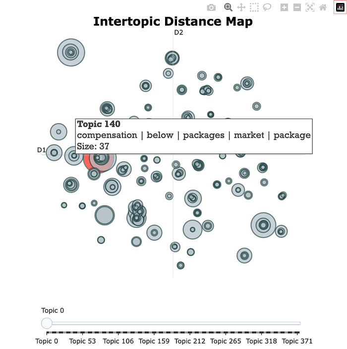
5. Extract Representative Documents
I next want to extract a handful of documents per each topic because it is too costly to send every document to an LLM API. In practice, you can often send much less information to an LLM provider than you’d expect and still get high-quality results. BERTopic’s built-in get_representative_docs() selects a subset of documents that best capture the key themes of each topic. The representative documents have the highest probabilities of belonging to their respective topics, acting like the “centroids” of the topic clusters in the 2D embedding space. These are what we will send to an LLM to get nice, human-friendly labels for all of our topics.
## bertopic.py ##

# Returns { topic_number: List[str] , ...}
rep_docs = bertopic_model.get_representative_docs()

rep_docs_df = pd.DataFrame.from_dict(rep_docs)
rep_docs_df.to_csv(
  f"../data/embeddings/representative_docs_{formatted_datetime}.csv",
  index=False
)
6. Label Topic Clusters with an LLM
After extracting the representative documents (rep_docs) from each cluster, the next step is to label the topic clusters. Here comes your opportunity to get good at prompt engineering. By sending only the rep_docs to an LLM, instead of every document in the corpus, we can drastically cut down time and cost while still getting accurate and descriptive topic labels and detailed topic descriptions.
One current limitation when making LLM calls is managing token limits. The code below tracks token count to make sure we don’t go over the model’s limit, while also formatting the input properly for the LLM.
The gen_prompt_text(input_str) function generates the formatted prompt that will be sent to the LLM for labeling and summarizing. Broadly, the function sets up some useful (and honest) context for the LLM, includes the pre-formatted input_str of rep_docs in the prompt, defines the task for the LLM to perform, handles edge cases / uncertainty, and returns the final prompt.
Here are some tips for prompt engineering:
- Provide Context: Contrary to current popular belief, it’s unnecessary to assign roles, such as telling the model that it is an “expert in x”, which is misleading. I find that performance improves when I honestly describe the problem I’m solving.
- Communicate Clearly: Test your prompt on a human. If they can’t understand what you are trying to achieve, refine the prompt until it’s easy for them to understand.
- Iteration: Run tests on a small sample of your corpus and iteratively improve the prompt. In my case, it took around 30 iterations before the prompt produced consistent results, though I still had occasional encounters with hallucination and the model randomly “going rogue”. (This happened mostly with the output structure I gave the model, not the topic labels themselves.)
- Format for Code: Use value placeholders in your output example rather than specific instances (see below).
- Give the LLM an Out: Sometimes the model is not confident in its response. If it can’t confidently find a topic, give it the option to say “No topic identified”.
- Be Polite and Honest: It’s a good heuristic to treat things well around you. And we don’t yet know what risks lie in not being polite and honest.
## llm.py ##
import tiktoken
import json

from functions.utils import get_llm_client # call to your chosen LLM provider

CONTEXT = (
    "I have a dataset of employee reviews about compensation packages " +
    "at various companies. The feedback consists of free-text responses, " +
    "ranging from short comments to detailed reviews."
)

TEXT_DELIMITER = '####'

# Change this to your model's context length
MODEL_CONTEXT_LENGTH = 4000

TOKEN_LIMIT = MODEL_CONTEXT_LENGTH - 256 # 256 is taken from the prompt token length


def count_tokens(string: str, encoding_name: str) -> int:
    """
       Returns the number of tokens in a text string
       e.g. "i love your t-shirt" -> 5
    """
    encoding = tiktoken.get_encoding(encoding_name)
    return len(encoding.encode(string))


def generate_prompt_text(input_str: str) -> str:
    """
      Generates the full prompt text
    """
    # 256 tokens in prompt without input_str
    user_message = f'''
    Below is a representative set of customer feedback comments delimited with {TEXT_DELIMITER}.

    Please identify the single main topic mentioned in these comments. Return a topic name and topic description.
    The topic name should be short, but descriptive.
    The topic description should not be a complete sentence. A good topic description looks like this:
    "Concerns about fair compensation compared to market rates"

    Return the topic name and description as a python dictionary with a single key-value pair like this:

    {{"topic_name": "<topicName>", "topic_description": "<topicDescription>"}}


    If you cannot find a good topic label, just say, "No topic identified".

    Employee feedback:
    {input_str}
    '''
    return CONTEXT + user_message


# prepare input_collections
input_collections = {}
results = {}

ENCODING_NAME = 'cl100k_base'

# rep_docs is a dictionary with key
for topic_int, topic_rep_docs_list in rep_docs.items():
    # join all topic rep_docs with a delimiter
    topic_rep_docs_string = TEXT_DELIMITER.join([
      str(x) for x in topic_rep_docs_list
    ])

    input_collections[f"{topic_int}"] = {
        "s": topic_rep_docs_string,
        # token count of string, if needed for token limit
        "t": count_tokens(topic_rep_docs_string, ENCODING_NAME)
    }

# Pass representative docs to LLM
for topic_int, prompt_obj in input_collections.items():
    prompt_text = generate_prompt_text(prompt_obj["s"])
    try:
        gpt_res = get_llm_client(prompt_text) # this is up to you to connect to your chosen LLM provider
        results[topic_int] = gpt_res
    except Exception as e:
        print(f"Failed to process topic {topic_int} with error: {e}")
        pass


# Save results
with open(f'../data/topics/prompt_results_{formatted_datetime}.json', 'w+') as fpout:
    json.dump(results, fpout)

print("Written to file")
7. Review / Reinforce / Repeat
The next logical step is to review the model’s performance and make improvements where necessary. More importantly at this stage though is to apply the model on new data to see if it generalizes well on something it has not seen before. Earlier we saved the model locally using the joblib package. Now it’s time to re-load it. You’ll need to process new data similarly to how you processed the original data (generating embeddings and normalizing them). Below is an example workflow:
## new_data.py ##

# Load model & new data
bertopic_model = joblib.load(
  f"../models/bertopic_model_{formatted_datetime}.joblib"
)
new_docs = [
  "New employee feedback 1",
  "Another new feedback comment, blah, blah",
  "Even more feedback data..."
]

# Repeat same embedding and pre-processing steps from above on new_docs...

# Apply the model to new data
new_topics, new_probs = bertopic_model.transform(
  new_docs,
  new_embeddings_normalized
)
You may want to periodically re-train your model if you expect topics to change significantly over time. In that case, you can re-train the BERTopic model with a combination of old and new data.

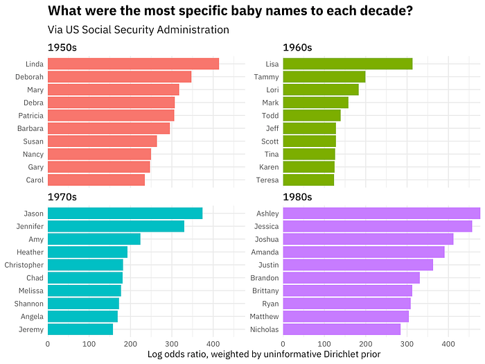
8. Weighted Log-Odds
With a full dataset of labeled topics and categorical features, the first instinct is to create bar charts of the most frequent topics by categories like sentiment or another feature. I am here to tell you not to waste your time doing this! A more insightful technique I learned from my coworker, data scientist and linguist Kate Lyons, is weighted log-odds (WLO).
Using a python adaptation of the WLO function from R’s tidylopy package by Julia Silge (via the tidylopy library), you can extract the most unique words per category, rather than just the most frequent ones. This is especially useful when you’re analyzing categories like sentiment, where common frequent topics might appear across both positive and negative sentiments, making it hard to discern what’s actually distinctive.
Weighted log-odds highlight the words that are the most specific or unique to a category and differentiate that category from others. See a few examples below.

¹ DALL-E 3 prompt to generate cover image: “A 2D t-SNE embedding space with thicker yarn points, forming more obvious clusters on a white background. The points are made from intertwined strands of yarn in bold purples, blues, oranges, reds, and pinks. The clusters are clearly distinct, with some regions densely packed with yarn points and others more spaced out. The thicker yarn creates a strong visual presence, making the clusters stand out while maintaining a soft, textured appearance. The arrangement reflects relationships and distances in the embedding space with a vibrant design, now contrasted against a clean white background.”
Thank you Charlie Oxborough for the coding collab and proofreading.